Tutorial 2: the Solow model
We are going to dig into into the seminal model of growth theory in macroeconomics: the Solow model.
Quick model summary
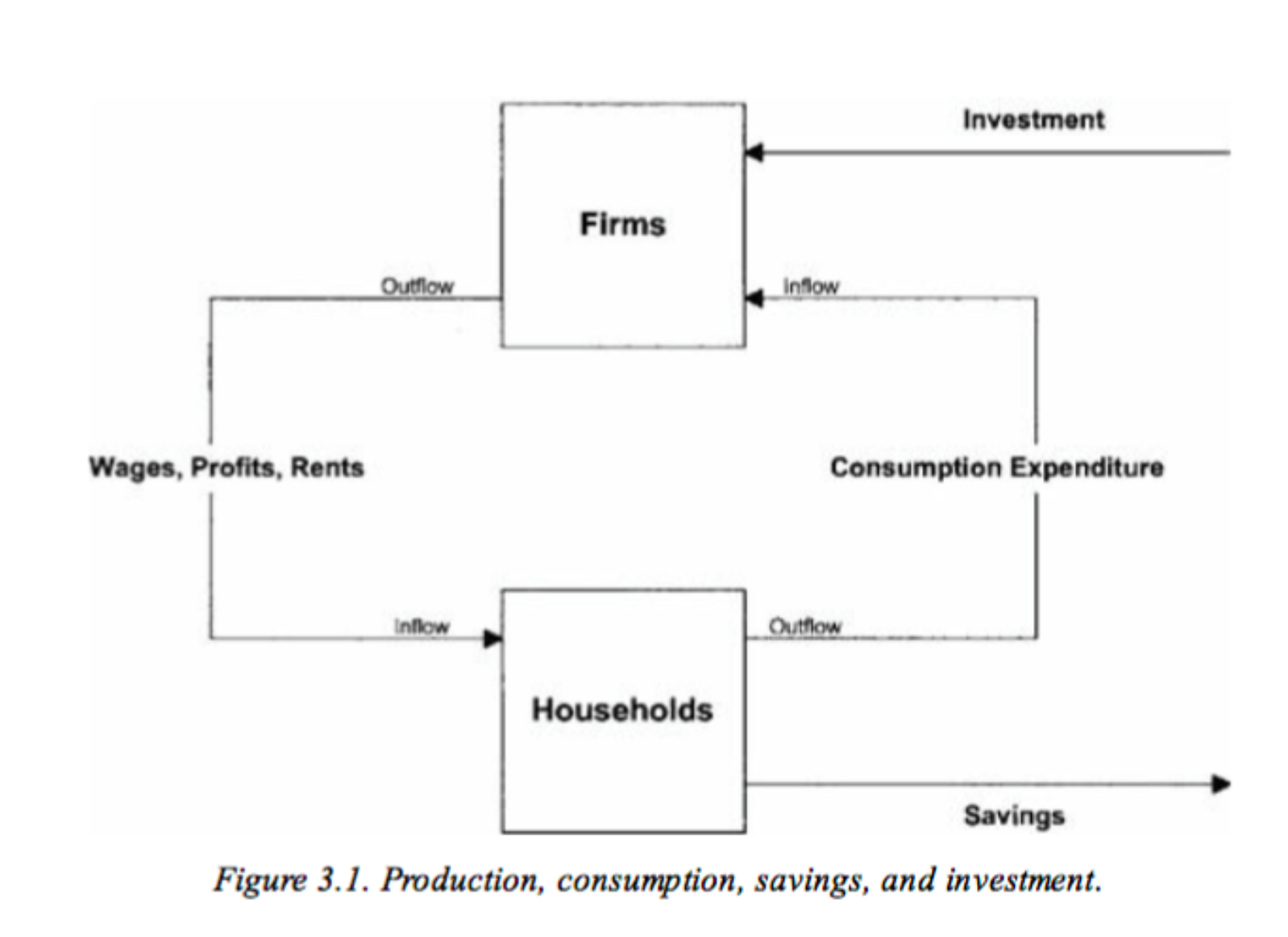
Structure of the economy: firms and consumers (no state). Firms use (and pay) capital and labor to produce an output. Output (=income) is either consumed or saved by households:
\[ Y_t = C_t + I_t \]
Production Function: a representative firm produces output using a Cobb-Douglas production function: \[ Y_t = F(K_t, A_tL_t) = K_t^\alpha (A_tL_t)^{1-\alpha}\] where \(Y\) is output, \(K\) is capital, \(L\) is labor and \(A\) is technology. where \(0 < \alpha < 1\). Using capital comes at rental price \(r\) and labor comes at price \(w\) (the wage).
Capital accumulation: capital accumulates through savings and depreciates geometrically
\[ K_{t+1} = I_t + (1-\delta) K_t\]
Saving rate: investment is a constant fraction of output
\[ I_{t} = sF(K_t,A_tL_t)\]
Definitions
- Steady state: trajectory where all variables are constant
- Balanced growth path: trajectory such that per capita variables grow at a constant rate (not necessarily the same) and the capital to output ratio is constant
Exercise
1. Warm-up: Return to scale
Let \(\lambda > 1\), if \(F(\lambda X, \lambda Y) < \lambda F(X,Y)\), the function has decreasing return to scales (and increasing for \(>\)). If \(F(\lambda X, \lambda Y) = \lambda F(X,Y)\), the function has constant return to scale. For the following functions, state if they exhibit positive, constant, or negative return to scale.
- \(y_1 = 10x^2y^2\)
- \(y_2 = \frac{1}{2}x^{1/3}y^{1/2}\)
- \(y_3 = x + 2y\)
- \(y_4 = \ln(xy)\)
2. Solve the firm’s maximization problem
Consider the function above (\(Y_t = K_t^{\alpha} (A_tL_t)^{1-\alpha}\)).
- Show that if \(K=0\) and/or \(L=0\) production does not occur
- Show that the production function has constant return to scale
- Show that marginal productivity is positive for capital and labour
- Show that marginal productivity is decreasing for capital and labour
- Write the down the profit maximization program (maximizing profit with respect to K and L) and derive its first order conditions
- Show that all output is needed to pay capital and labor
3. Constant population and technology
For now, we consider that technology and labor (=population) are constant (\(A_t = A\), \(L_t = L\)): no population growth, no technological progress.
- Using the capital accumulation equation, show that the ratio \(\frac{K_{t+1}}{K_t}\) goes to \(\infty\) as \(K_t\) goes to 0 and is lower than 1 when \(K_t\) goes to \(\infty\)
- Show that there is a unique steady state level of capital \(k^*\) and solve for it
- How does the \(k^*\) vary with \(s\), \(\delta\), \(A\), \(L\) ? Interpret
4. Population and technology growth
We now assume that population grows at constant rate \(n\), and technology at rate \(g\):
\[L_{t+1} = (1+n) L_t\]
\[A_{t+1} = (1+g) A_t\]
We respectively denote \(y_t=Y_t/L_t\) and \(k_t=K_t/L_t\), the per-worker production and capital
We further define \(\hat{y_t}=\frac{Y_t}{A_t L_t}\) and \(\hat{k_t}=\frac{K_t}{A_tL_t}\) the production and capital per effective unit
Dividing the capital accumulation equation by \(A_tL_t\), show that
\[\hat{k_{t+1}} (1+n)(1+g)= (1-\delta)\hat{k_t} + s F(\frac{K_t}{A_tL_t},1)\]
Show that there is a steady state level of capital per effective unit \(\hat{k^*}\) equal to:
\[ \hat{k^*} = \left(\frac{s}{(1+n)(1+g)-1+\delta}\right)^{\frac{1}{1-\alpha}} \]
- Show that per capita outcomes \(y\) and \(k\) are on a balanced growth path. What is their respective growth rates?
5. Discussion
- What makes this model a simplification of reality?
- Why cannot it explain all differences in output growth and per capita level across economies?